Interpreting the results

pyorbit_results will produce several files depending on the flags provided at runtime. The following sections will provide you with a detailed description.

Documentation update!

This page was updated on October 2024 to reflect the updates of version 10 of PyORBIT.

Confidence intervals

Confidence intervals and/or associated errors are computed using the 15.865th and the 84.135th percentile of the distribution. The median value of the distribution (50th percentile) is then subtracted from these two values. For clarity, these values are always followed by the string (15-84 p). The following values:

----- dataset:  RV_data
jitter_0                  2.04        -0.34         0.35    (15-84 p)

read as \(\mathrm{jitter}_0 = 2.04_{-0.34}^{+0.35} \, ms^{-1}\), or equivalently \(\mathrm{jitter}_0 = 2.04 \pm 0.35 \, ms^{-1}\)

Note

The code will format the output according to the significant figures of a measurement. The unformatted value can always be retrieved from the posterior distribution. In case of reparametrisation, please be sure to use the correct posterior distribution.

The associated error is not provided for the starting point of the MCMC analysis, the MAP values, fixed values, or, in general, when the percentile of the distribution cannot be computed.

Terminal output

The terminal output will produce a detailed summary of the analysis. It cannot be turned off, but you can easily redirect the output to a log text file:

pyorbit_results emcee my_file.yaml -all > my_file_emcee_res.log 

First thing you will get is a list of a few characteristics of your system. This section may change depending on your computer configuration and the employed sampler.

PyORBIT v10.6.3

Python version in use:
3.10.14 (main, May  6 2024, 19:42:50) [GCC 11.2.0]

LaTeX disabled by default

emcee version:  3.1.6

 Reference Time Tref: 56456

 Dimensions = 21
 Nwalkers = 84

 Steps: 50000

If you use the -all flag, you will get several log messages regarding the status of plot preparation and plot printing. Those are detailed in the corresponding section.

Basic model selection

The code provides the log-probability value, with its two components (the log-priors and the log-likelihood) explicitly reported right below.

 LN posterior:  -419.758906      -4.028171     3.223933 (15-84 p) 

 Median log_priors     = -27.54775920683063
 Median log_likelihood = -381.9071666017402

The error associated to the log-probability is computed

The code computes the Bayesian Information Criterion (BIC), the Akaike Information Criterion (AIC) and the AIC with a correction for small sample sizes (AICc). These values are computed using the median value of the log-probability / log-likelihood. These three criteria should be computed using the log-likelihood, but I’ve seen several cases where the log-probability is used instead. The appropriate choice is left to the user.

 Median BIC  (using likelihood) = 895.0232335681574
 Median AIC  (using likelihood) = 805.8143332034804
 Median AICc (using likelihood) = 807.680999870147

 Median BIC  (using posterior)  = 950.1187519818186
 Median AIC  (using posterior)  = 860.9098516171416
 Median AICc (using posterior)  = 862.7765182838083

The maximum a posteriori (MAP) set of parameters is computed by picking the sampling corresponding to the maximum value of the log-probability distribution. As in the previous steps, different model selection criteria using either the log-likelihood or the log-probability are reported here, with the difference that now the corresponding MAP value is used rather than the corresponding median value.

 MAP log_priors     = -27.937645542438936
 MAP log_likelihood = -383.0025104725866

 MAP BIC  (using likelihood) = 897.2139213098502
 MAP AIC  (using likelihood) = 808.0050209451732
 MAP AICc (using likelihood) = 809.8716876118399

 MAP BIC  (using posterior)  = 953.0892123947281
 MAP AIC  (using posterior)  = 863.8803120300511
 MAP AICc (using posterior)  = 865.7469786967177

Finally, the code suggests the use of either AIC or AICc according to the standard definition

 AICc suggested over AIC because NDATA ( 517 ) < 40 * NDIM ( 21 )

Warning

No check over BIS/AIC/AICc statistical validity is performed! Be sure that the underlying assumptions are valid in your specific case.

Autocorrelation analysis

If the posteriors have been computed using an MCMC sampler, as emcee, an autocorrelation analysis is performed automatically using the methods implemented in the sampler. For more information, please check the Autocorrelation analysis and convergence page from the emcee documentation.

Important

The sampler chains used to compute the ACF include the burn-in values.

PyORBIT will first compute the integrated autocorrelation time for each variable using the built-in method in emcee. This method automatically checks if the chains are long enough for a reliable autocorrelation analysis. If everything is fine, you’ll get this message:

The chains are more than 50 times longer than the ACF, the estimate can be trusted

If the chains are too short, the tolerance parameter (i.e., the minimum number of autocorrelation times needed to trust the estimate) will be lowered to 20, with a warning and a (likely overestimated) suggestion for the appropriate chain length.

***** WARNING ******
The integrated autocorrelation time cannot be reliably estimated
likely the chains are too short, and ACF analysis is not fully reliable
emcee.autocorr.integrated_time tolerance lowered to 20
If you still get a warning, you should drop these results entirely

Chains too short to apply convergence criteria
They should be at least 2800*nthin = 280000

The maximum value of the integrated time is then used as step length (or step size) in the following analysis.

Computing the autocorrelation time of the chains
Reference thinning used in the analysis: 100
Step length used in the analysis: 14*nthin = 1400

The convergence criteria are clearly stated for your benefit. After discarding the first `tolerance’ steps, the relative variation between two consecutive steps must be lower than 0.01 (1%). The 1% criterion must be satisfied five times before validating the convergence to avoid underestimating convergence time due to statistical variations.

Convergence criteria: less than 1% variation in ACF after 50 times the integrated ACF
At least 50*ACF after convergence, 100*ACF would be ideal
Negative values: not converged yet

Finally, you’ll get a (badly formatted) table to identify misbehaving variables, and a suggestion regarding the number of steps required to satisfy the criterion reported above for each parameter.

sampler parameter	ACF	ACF*nthin	converged at	nsteps/ACF	to 100*ACF
RVdata_jitter_0	4.94	494	27600	45	26976
RVdata_offset_0	5.45	545	30000	37	34504
BISdata_jitter_0	4.92	492	26400	48	25600
BISdata_offset_0	4.81	481	32400	37	30533
…	…	…	…	…	…

Legend:

• sampler parameter: the parameter explored by the sampler (it may be different from the parameter of the model)

• ACF: the integrated autocorrelation time computed on the thinned chains.

• ACF*nthin: the integrated autocorrelation time in units of sampler steps

• converged at: number of sampler steps at which the chain converged

• nsteps/ACF: number of steps in unit of ACF performed after reaching convergence

• to 100*ACF: number of steps required to reach a length equal to 100 times the ACF

The code provides the average estimate of additional steps required to reach 50 times and 100 times the ACF lenght.

All the chains have converged, but PyORBIT should keep running for about:
53068 more steps to reach 50*ACF,
27186 more steps to reach 100*ACF

The average is computed over the parameters that have yet to cross those thresholds. It’s important to note that misbehaving parameters can significantly influence these suggestions towards higher values. Before blindly relaunching the analysis to reach the suggested value, a visual inspection of the chains may help determine whether continuing with the analysis is a worthy investment of time.

The suggested value for the burn-in is computed as the average value of the convergence point of each parameter:

Suggested value for burnin: 42067

Two rows of asterisks delimit the end of this section.

Skewed posteriors and their effects on the ACF

In my empirical experience, parameters with posterior distribution significantly deviating from a Normal distribution may result in unreliable values for the ACF and the convergence point. Let’s take the outcome of a fit of a lightcurve as an example:

sampler parameter	ACF	ACF*nthin	converged at	nsteps/ACF	to 100*ACF
b_P	4.44	444	28000	162	0
b_R_Rs	5.05	505	29400	140	0
b_sre_coso	5.02	502	28700	142	0
b_sre_sino	6.18	618	35700	104	0
b_b	7.87	787	44800	70	23547
b_Tc	4.24	424	26600	173	0

All the planetary parameters were sampled for a number of steps greater than 100 times the ACF, except for the impact parameter. This is the automatic suggestion you get from PyORBIT:

All the chains are longer than 50*ACF, but some are shorter than 100*ACF
PyORBIT should keep running for about 23547 more steps to reach 100*ACF
Suggested value for burnin: 30362

We can have a look at the trace plot (also referred as chain plot) to visually inspect if convergence has been reached:

Fig. 1 Chain plot as a function of thinned iteration number (step) for the impact parameter. Each color identifies a different walker.

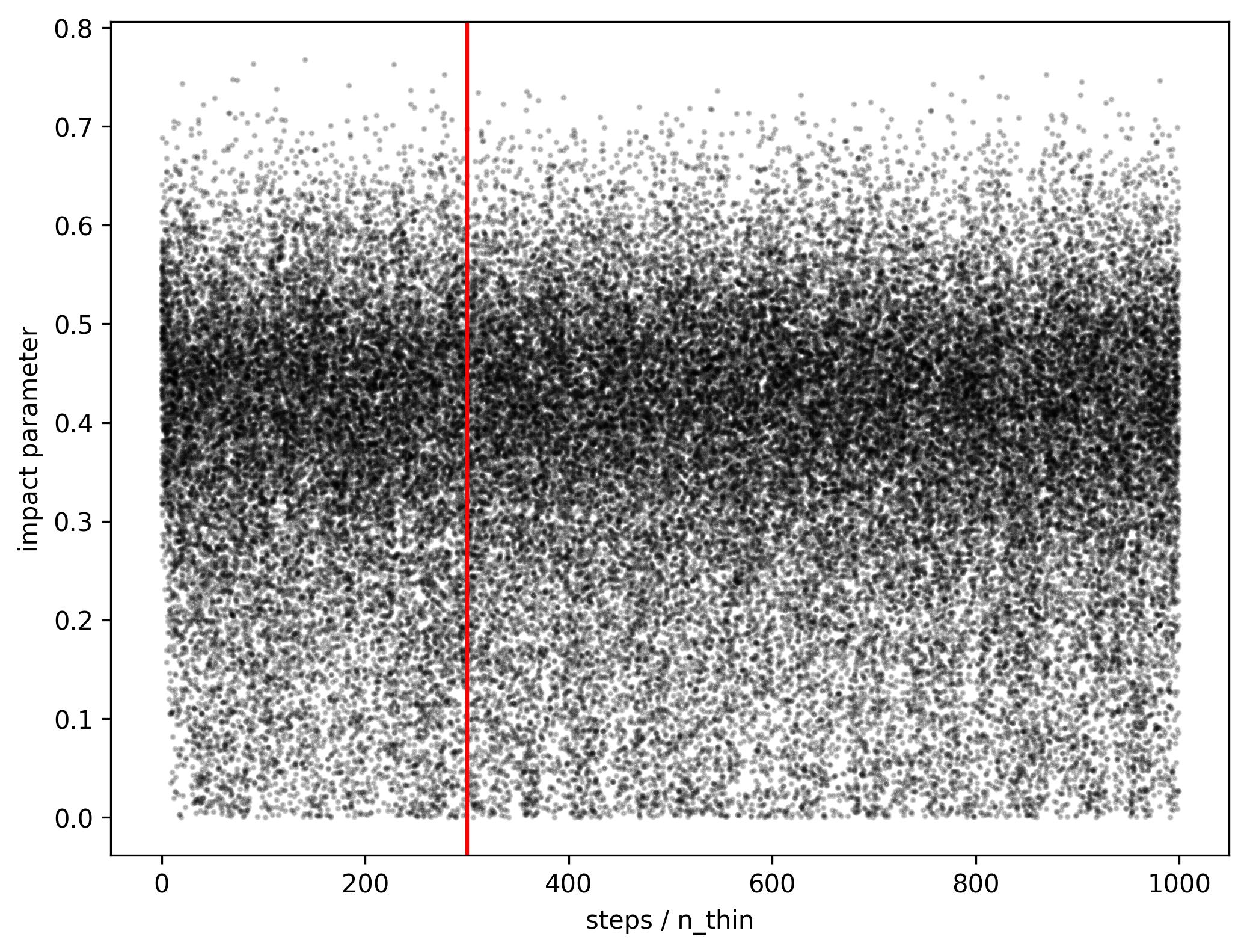
Fig. 2 The same data as the above plot, this time using dots to show the parameter distribution as a function of the thinned iteration number.

To further check if the chain has converged, i.e., if the parameter has reached a stationary distribution independent of the lenght of the chain, we can plot the parameter distribution for ranges of 100 thinned steps.

Fig. 3 Parameter distribution for different ranges of thinned iteration numbers.

Even if the ACF tells us differently, we don’t have any reason to believe that the chain has not already converged at 200/300 thinned steps.

In conclusion, the ACF provides reliable results most of the time. When ACF convergence warnings are restricted to a few parameters, a simple visual inspection or an independent check of the chains’ behaviour may be sufficient.

Confidence intervals of the parameters

Confidence intervals of the posteriors are provided at 34.135th percentiles from the median on the left and right sides, in addition to the median, as specified in the previous section.

This section is divided into three groups:

• Statistics on the posterior of the sampler parameters: the direct output of the sampler. If the parameters have been parametrised (including exploration in logarithmic space), the values displayed here may not be physically meaningful.

• Statistics on the model parameters obtained from the posterior samples: confidence intervals of the model parameters (i.e., before reparametrisation) as they should appear in the physical model. If no reparametrisation has been applied to a given parameter, the model posterior will be identical to the sampler posterior.

• Statistics on the derived parameters obtained from the posterior samples: confidence intervals of those parameters that are not directly involved in the optimisation procedure, but are derived from the model parameters through an analytical transformation.

The scheme will be repeated two times: once to print the confidence intervals of sampler/model/derived parameters, and again, to print the corresponding MAP values.

Let us take an example involving the determination of a planetary radius through light curve fitting:

Statistics on the posterior of the sampler variables

====================================================================================================
     Statistics on the posterior of the sampler variables
====================================================================================================

----- common model:  b
P                0       3.54233     -0.00021      0.00019   (15-84 p)   [    3.4402,     3.6402]
R_Rs             1        0.0423      -0.0013       0.0013   (15-84 p)   [    0.0000,     0.5000]
sre_coso         2          0.00        -0.21         0.21   (15-84 p)   [   -1.0000,     1.0000]
sre_sino         3          0.03        -0.21         0.18   (15-84 p)   [   -1.0000,     1.0000]
b                4          0.39        -0.19         0.12   (15-84 p)   [    0.0000,     2.0000]
Tc               5  2459474.8566      -0.0013       0.0014   (15-84 p)   [2459473.1000, 2459475.1000]

When reporting the sampler results, the name of the parameter is followed by a number indicating its position in the array of parameters passed to the optimization algorithm. These numbers are for internal use only (they my change from run to run), but they can be useful to check the dimensionality of the problem. At the end of the line, the boundaries of the parameters are reported: these boundaries can be assigned by the users (as in the case of P and Tc) or internally defined (as for b and R_Rs).

In this example you can see that the orbital period P is negative: this is not an error, as the parameter is being explored in logarithmic space (specifically, Log2) and not in Natural base. Note also that eccentricity \(e\) and argument of pericenter \(\omega\) are parametrized as \(\sqrt{e} \sin \omega\) (sre_sino) and \(\sqrt{e} \cos \omega\) (sre_coso) following Eastman et al. 2013. I should make priors and spaces more explicit at output

Statistics on the model parameters obtained from the posterior samples

====================================================================================================
     Statistics on the physical parameters obtained from the posterior samples
====================================================================================================

----- common model:  b
P                      3.54233     -0.00021      0.00019    (15-84 p)
R_Rs                    0.0423      -0.0013       0.0013    (15-84 p)
b                         0.39        -0.19         0.12    (15-84 p)
Tc                2459474.8566      -0.0013       0.0014    (15-84 p)
e                        0.061       -0.042        0.059    (15-84 p)
omega                     -147         -117          139    (15-84 p)

The main difference concerning the previous table is that the columns of the parameter index and the parameter boundaries are not listed here, as not all the parameters may have been directly involved in the optimisation procedure. The orbital period P is now expressed in the correct unit (days) as it has been converted from logarithmic to natural space, while the other parameters b, Tc, and R_Rs are identical as they did not go through any transformation. The argument of pericenter (omega) and the eccentricity e are now explicitly reported, as they are the actual parameters of the physical model.

In the case of a circular orbit, sre_sino and sre_coso would not be listed in the sampler parameters output, while the eccentricity e and the argument of periastron \omega would be listed as fixed parameters and without confidence interval, as the model still requires these terms, although they are not involved in the optimisation procedure.

...
e                 0.000000e+00
omega                90.000000
...

Statistics on the derived parameters obtained from the posteriors samples

====================================================================================================
     Statistics on the derived parameters obtained from the posteriors samples
====================================================================================================

----- common model:  b
a_Rs                     11.28        -0.19         0.19    (15-84 p)
i                        88.01        -0.52         0.95    (15-84 p)
mean_long                 71.2         -7.0          7.0    (15-84 p)
R_Rj                     0.339       -0.011        0.011    (15-84 p)
R_Re                      3.80        -0.12         0.12    (15-84 p)
T_41                    0.0967      -0.0052       0.0051    (15-84 p)
T_32                    0.0875      -0.0060       0.0059    (15-84 p)
a_AU_(rho,R)           0.04320     -0.00082      0.00080    (15-84 p)

This table looks a lot like the physical parameters table, the main difference with the difference that these values are either obtained though internal transformation of the physical parameters, as in the case of the scaled semi-major axis a_Rs or the orbital inclination i, or using some external parameters, as the planetary radius in Jupiter radii R_Rj and Earth radii R_Re, both requiring a prior on the stellar radius which is however not involved in the optimization procedure.

Differences between MCMC and nested sampling outputs

The output described above applies to MCMC samplers. Nested sampling algorithms will have slightly different output:

• Autocorrelation function analysis will not be performed.

• An extra step reporting the boundary of the parameters will be printed.

• A short summary with the confidence interval for the Bayesian evidence may be printed.

• Some additional plots may be produced according to the methods implemented in the specific sampler.

The additional outputs follow closely the examples reported in the documentation of each sampler, so they will not be detailed here.

Note on reparametrisation and transformation of parameters

Median values and confidence intervals for the model and derived parameters are computed directly on the transformed posterior, rather than on the reported values for the sampler parameters. In other words, each set of parameters from the posterior distribution is converted into the model/derived parameters, generating a new distribution for each new parameter, then the median and the confidence intervals are computed on newly generated distribution. For this reason, the median of a model parameter may not correspond to the direct conversion of the median of the sampler parameters. Using the example shown before:

\[\begin{split}\sqrt{e} \sin{\omega} = 0.03 \\ \sqrt{e} \cos{\omega} = 0.00\end{split}\]

\[e_{\mathrm{sampler}} = (\sqrt{e} \sin{\omega})^2 + (\sqrt{e} \cos{\omega} )^2 = 0.0009\]

while the reported median value for the eccentricity in the model parameters section is (correctly) \(e = 0.061\).