Simultaneous GPs on photometry and spectroscopy#
Imagine we have both photometric and spectroscopic time series of a rather active star. Photometry will provide essential information on the rotational period of the star and the decay time scale of activity regions, while spectroscopic activity indexes are essential to disentangle planetary and stellar signal in radial velocities.
In this example, we will analyze the planetary system around K2-141 Malavolta et al. 2018. The spectroscopic dataset is taken from Bonomo et al. 2023 and includes Radial velocity data, Bisector Inverse Span, and S-index, all gathered with HARPS-N.
Photometric data comes from K2 campaign 12, corrected fro systematics as described in Vanderburg and Johnson 2014 and available at the MAST K2SFF website. Data from TESS sector 42 and sector 70 are available, but we are not going to use them in this example.
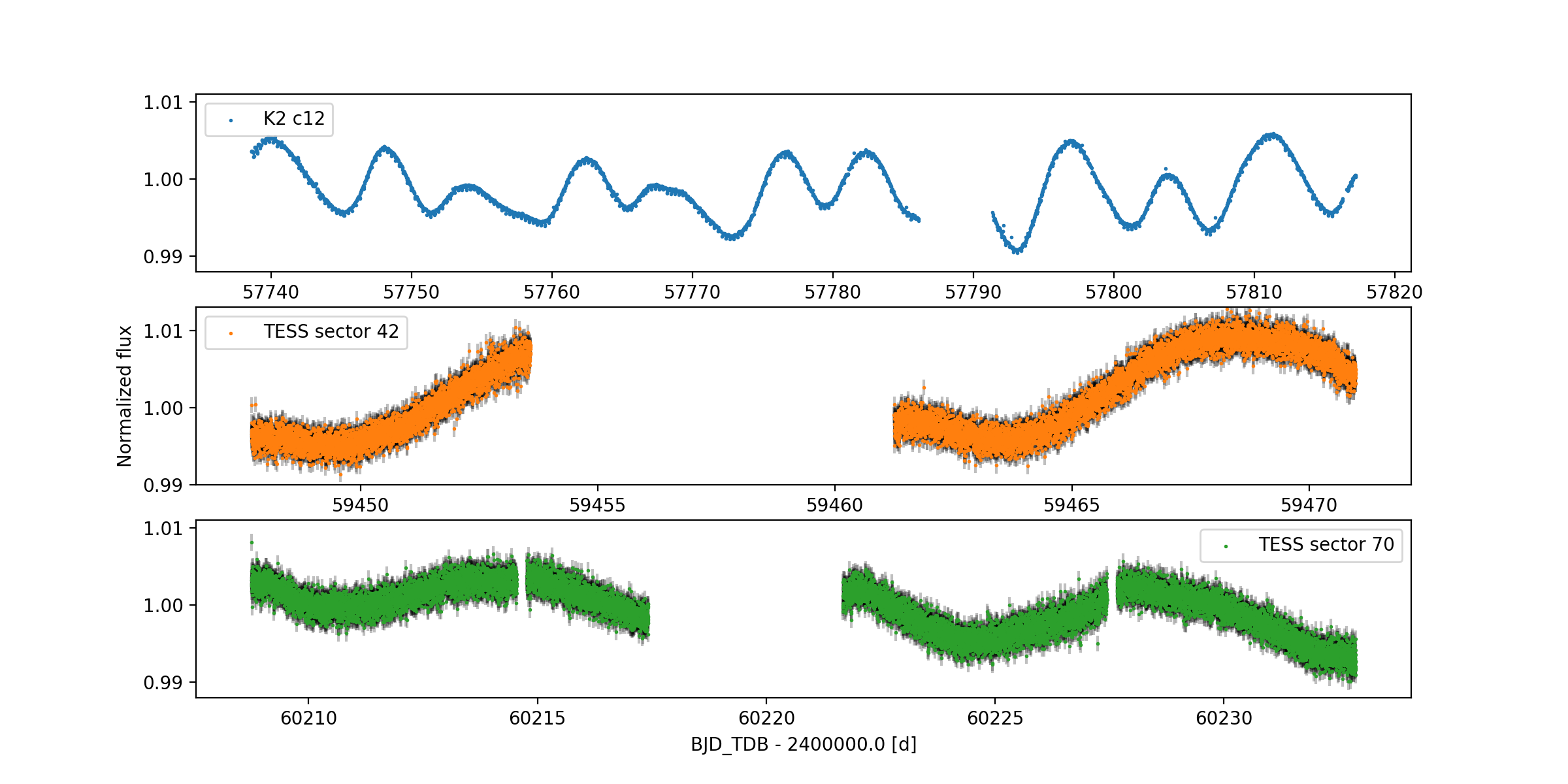
Fig. 4 Photometric data for K2-141. The stellar activity modulation is clearly identifiable.#
We want to model stellar activity in photometry simultaneously with the spectroscopic time series.
For photometric data, we use the [exponential-sine periodic kernel] (ESP) implemented in ‘S+LEAF’. Each dataset will have its independent covariance matrix.
For spectroscopic data, we use the multidimensional quasi-periodic kernel through
tinygp.
For the photometric data, we also include the transit model for the two planets, and a normalization factor, independent for each dataset (if you have more than one light curve). Check the Light curve fit section in Quickstart for additional information.
For the spectroscopic data, we only have to include the radial_velocities model due to the planets in the radial velocity dataset.
The input section takes this form:
 1inputs:
 2  LC_K2_c12:
 3    file: datasets/K2-141_K2_KSFF_PyORBIT.dat
 4    kind: Phot
 5    models:
 6      - spleaf_esp
 7      - lc_model
 8      - normalization_factor
 9  RVdata:
10    file: datasets/K2-141_RV_PyORBIT.dat
11    kind: RV
12    models:
13      - radial_velocities
14      - gp_multidimensional
15  BISdata:
16    file: datasets/K2-141_BIS_PyORBIT.dat
17    kind: BIS
18    models:
19      - gp_multidimensional
20  Sdata:
21    file: datasets/K2-141_Sindex_PyORBIT.dat
22    kind: S_index
23    models:
24      - gp_multidimensional
In the common section, we specify:
the two transiting planets:
planets:bandplanet:c. Note that we do not specify any prior on the period or transit time, as they will be fitted directly in photometric data;activity: the rotational period of the star
Prot, the decay timescale of activity regionsPdec, and the coherence scaleOamp, will be shared among the trained ESP and the multidimensional QP.stellar parameters: in addition to he priors on mass, radius, and density, we also include priors on the limb darkening coefficients for the two instruments involved in our analysis;
25common:
26  planets:
27    b:
28      orbit: circular
29      use_time_inferior_conjunction: True
30      boundaries:
31        P: [0.2750, 0.2850]
32        K: [0.001, 20.0]
33        Tc: [57744.00, 57744.10]
34      spaces:
35        P: Linear
36        K: Linear
37    c:
38      orbit: keplerian
39      parametrization: Eastman2013
40      use_time_inferior_conjunction: True
41      boundaries:
42        P: [7.70, 7.80]
43        K: [0.001, 20.0]
44        Tc: [58371.00, 58371.10]
45        e: [0.00, 0.70]
46      priors:
47        e: ['Gaussian', 0.00, 0.098]
48      spaces:
49        P: Linear
50        K: Linear
51  activity:
52    boundaries:
53      Prot: [10.0, 20.0]
54      Pdec: [20.0, 1000.0]
55      Oamp: [0.001, 1.0]
56  star:
57    star_parameters:
58      priors:
59        mass: ['Gaussian', 0.708, 0.028]
60        radius: ['Gaussian', 0.681, 0.018]
61        density: ['Gaussian', 2.65, 0.08]
62    limb_darkening:
63      type: ld_quadratic
64      priors:
65        ld_c1: ['Gaussian', 0.68, 0.10]
66        ld_c2: ['Gaussian', 0.05, 0.10]
In the models section we include two models for Gaussian Process regression: the spleaf_esp will perform GP regression on each light curve independently (if you have more than one light curve), i.e., each light curve will have its own covariance matrix and its own amplitude of the covariance, similarly when performing the trained GP regression.
The gp_multidimensional will perform multidimensional GP regression over the datasets that are employing these model, namely for this specific example, the RV dataset, the BIs dataset, and the S index.
You may notice that both spleaf_esp and gp_multidimensional are recalling the same common model common:activity. The GP hyperparameters will be shared, in this sense we may say that photometry is training the hyperparameters of the multidimensional GP.
 67models:
 68  radial_velocities:
 69    planets:
 70      - b
 71      - c
 72  lc_model:
 73    kind: pytransit_transit
 74    limb_darkening: limb_darkening
 75    planets:
 76      - b
 77      - c
 78  normalization_factor:
 79    kind: local_normalization_factor
 80    boundaries:
 81      n_factor: [0.9, 1.1]
 82  spleaf_esp:
 83    model: spleaf_esp
 84    common: activity
 85    n_harmonics: 4
 86    hyperparameters_condition: True
 87    rotation_decay_condition: True
 88    LC_K2_c12:
 89      boundaries:
 90        Hamp: [0.000, 1.00]
 91  gp_multidimensional:
 92    model: tinygp_multidimensional_quasiperiodic
 93    common: activity
 94    hyperparameters_condition: True
 95    rotation_decay_condition: True
 96    RVdata:
 97      boundaries:
 98        rot_amp: [-100.0, 100.0] #at least one must be positive definite
 99        con_amp: [0.0, 100.0]
100      derivative: True
101    BISdata:
102      boundaries:
103        rot_amp: [-100.0, 100.0]
104        con_amp: [-100.0, 100.0]
105      derivative: True
106    Sdata:
107      boundaries:
108        con_amp: [-1.0, 1.0]
109      derivative: False
The rest of the configuration file looks as usual.
129parameters:
130  Tref: 59200.00
131  safe_reload: True
132  use_tex: False
133  low_ram_plot: True
134  plot_split_threshold: 1000
135  cpu_threads: 32
136solver:
137  pyde:
138    ngen: 50000
139    npop_mult: 4
140  emcee:
141    npop_mult: 4
142    nsteps: 50000
143    nburn: 20000
144    nsave: 25000
145    thin: 100
146  recenter_bounds: True